Route/Tour Definition

CO2 Analysis

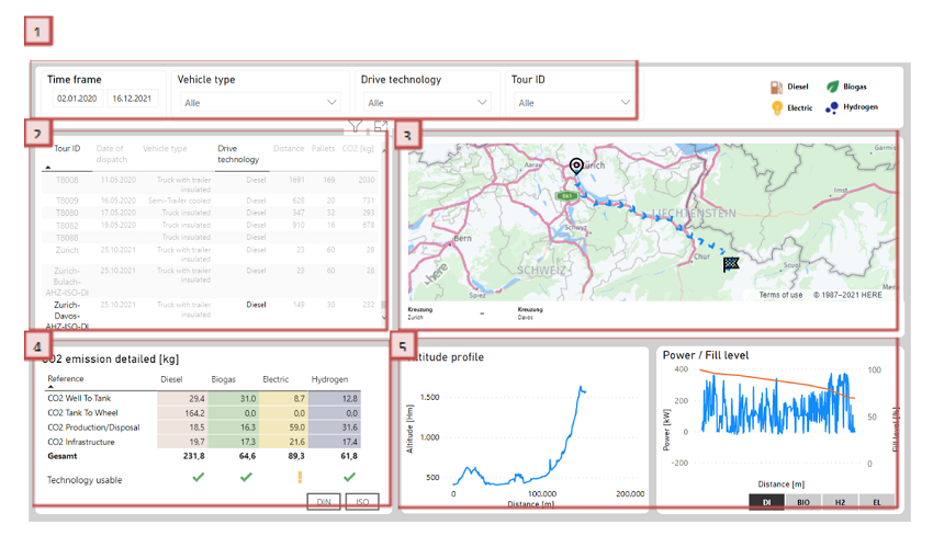
Page 1 (CO2 analysis) shows the results of the calculations on an individual tour basis. The subsequent analysis is based on this page.

1. All relevant filter options for the dashboard are set here. It can be filtered according to a specific time period, vehicle type, drive technology or tour ID. This filter logic applies to all pages in the dashboard.

2. All tours that meet the filter criteria under point 1 are displayed here. To activate the other visualizations on this page, a tour must be selected by clicking it once.

3. In this field, the start, intermediate and end points of the tour selected in point 2 are shown both in map form and in writing.

4. The table gives an overview of the emissions for all existing drive technologies across the different scopes. The available standards for emission calculation (ISO 14040 and DIN EN 16258) can be selected at the bottom right. The emission scopes can be differentiated as follows:

5. CO2 Well To Tank à Emissions that arise in the provision of the required energy “from the source to the vehicle tank”.

6. CO2 Tank To Wheel à Exhaust emissions or those emissions caused by the combustion of fuel.

7. CO2 Production/Disposal à The production, maintenance and professional disposal of a vehicle results in emissions that can be broken down into an individual tour. This is only relevant to the lifecycle view (ISO 14040).

8. CO2 Infrastructure à The use of infrastructure (e.g. roads) results in emissions that can be attributed to a vehicle when the vehicle is driven on it. This is only relevant to the lifecycle view (ISO 14040).

In addition to CO2 emissions, the table also shows which technology is suitable for the selected tour. If a green tick is shown, the tour should be possible without any problems. If a yellow exclamation mark is shown, the drivability of the tour is questionable. This could be due to the following reasons:

• The range of the vehicle is not sufficient to complete the tour with one tank load (based on the master data of the tank/battery size stored for the respective drive technology).

• The drive power requirements are either too high or very high over a long period of time, i.e. use could lead to overheating.

Due to technology developments and innovations, the master data used to assess the drivability of certain tours may be updated from time to time.

1. The elevation profile (left) and the engine performance requirements (right) over the course of a tour are shown here. The theoretical fill level of a tank/battery is also calculated and shown.

CO2 balance sheet

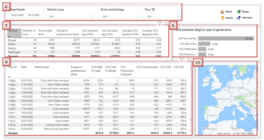
Page 2 shows the calculated tours in consolidated and summarized form.

1. The filter logic is as described in point 1.

2. The total of all calculated tours that meet the filter criteria under (1) is shown here. In addition to the total CO2 emissions, key figures such as transport performance (km/tkm) are also shown. The total CO2 emissions are expressed in relation to the transport performance in order to supplement the absolute total with a relative key figure. A distinction is made according to the drive technology used.

3. The total CO2 emissions are broken down here according to the different scopes (described in point 4).

4. All calculated tours are listed again here and supplemented with the transport performance (tkm). By clicking on a tour, all figures shown (points 7, 8, 10) are adjusted so that only the values for the selected tour are visible.

5. By clicking on a tour (point 9), a map view is made available.

CO2 Balance Sheet Development

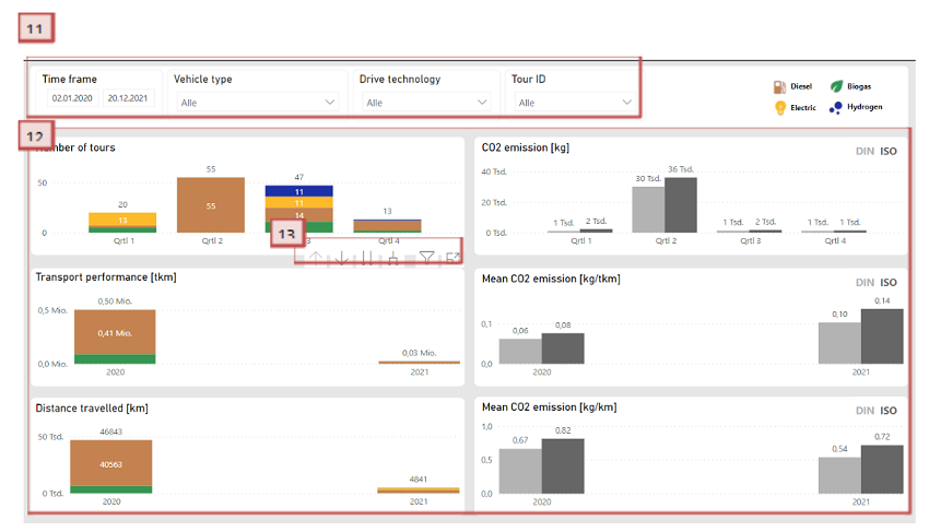
On page 3, the calculated data is supplemented and analyzed from a time perspective.

1. The filter logic is as described in point 1.

2. Here, the values given on pages 1 and 2 are placed on a time axis. In addition to the number of tours and the transport performance (km/tkm), the CO2 emissions are also shown in absolute and relative terms (per km/per tkm).

3. The granularity of the time axis can be controlled for each graphic with the arrows framed here. The following is a brief description of the functionality of the navigation:

Up arrow: “Drill-up” / moves up one level of granularity

Down arrow: can be used to activate the “drill-down”

Double down arrow: moves down to the next lower level of granularity

Branched arrow: activates all elements of the next lower level of granularity

Funnel: shows all filters that affect the visualization

Picture in picture: enlarges the selected visualization

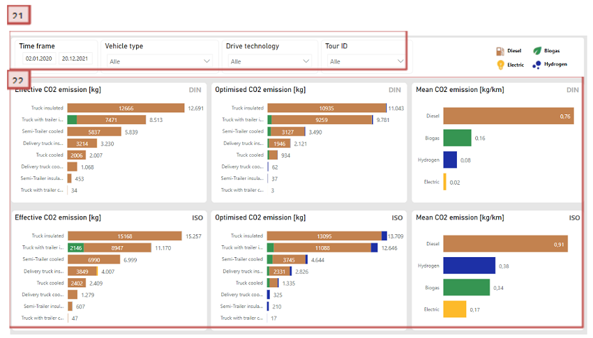
Potential Analysis DIN/ISO

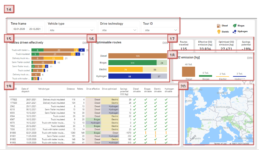
Pages 4 and 5 serve to outline the (CO2)-optimal vehicle fleet based on the calculations performed. Page 4 uses the DIN 16258 standard, whereas page 5 uses the ISO 14040 standard (lifecycle).

1. The filter logic is as described in point 1.

2. Here the number of tours driven with which drive technology is shown, broken down by vehicle category.

3. This visualisation shows how many of the calculated tours could have been driven with the available alternative drive technologies since the drivability test (point 4) was positive (dark colour = drivability OK / light colour = drivability needs to be checked). Clicking on the light portion for each drive technology (point 18) shows the tours that did not pass the drivability test without restrictions.

4. The key figures show how many tours were calculated, the actual level of CO2 emissions and what they would have been if the CO2-optimal drive technology that passes the drivability test had been used.

5. This shows the level of CO2 emissions if all tours had been driven with one of the available drive technologies.

6. This table shows which drive technology was actually used for each tour and which technology could have been used optimally. By clicking on a tour, all figures shown (points 15, 16, 17, 18) are adjusted so that only the values for the selected tour are visible.

7. By clicking on a tour (point 19), a map view is made available.

Potential Analysis Comparison

On page 6, the optimized and mean (relative) CO2 emissions of the two stored standards (ISO 14040 and DIN EN 16258) are compared.

1. The filter logic is as described in point 1.

2. Here, the actual, optimized and mean (relative) CO2 emissions of the two stored standards (ISO 14040 and DIN EN 16258) are compared according to vehicle category.

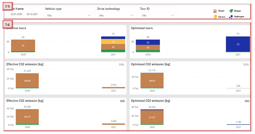
Potential Analysis Over Time

Optimizations are expressed on a time axis.

1. The filter logic is as described in point 1.

2. Actual and CO2-optimised route planning on a time axis. The functions described in point 13 are also available here.

Remarks:

The term CO2 always refers to CO2 equivalents. Other greenhouse gases (NOx, CH4, SO2, etc.) are also included here. Due to the different greenhouse effects, these are then converted to the equivalent effect of CO2.